Last week I was asked by a client how many requests per second his new web application could handle in the initial setup. Instead of a plain number I presented him the graph on the left and said:
»It depends«.
Without going too deep into
theory the throughput (responses per second in this case) depends on the number of items in the system (i.e. active TCP connections with a pending response) and cycle time (i.e. response time) in a operationalized variant of
Little's Law. So, to be more precise and applied to our current topic we get equation 1. Let's say we have an application with an average response time of 100ms and we use one connection that constantly requests a resource (for instance with
ApacheBench:
ab -c 1 -n 100 http://example.com/). According to Little's Law a benchmark like this will yield 10 requests per second*. With two connections the result should be 20 requests per second, with four connections 40 requests and so on. In short, as long as you do not reach the capacity limit of a system, the throughput doubles with with each doubling of connections (i.e. scales linearly with factor 1).
 |
| Equation 1: Operationalized Little's Law Applied to Web Applications |
 |
Checkin Terminals
at the Airport |
Now to the capacity limit. An illustrative example would be a check in terminal at the airport. Let's assume that the average checkin time is 1 minute and there are 10 terminals available for check in. Clearly, the maximum throughput will be 10 check ins per minute. But what happens if more as 10 customers arrive at the same time? The simple answer is: They have to wait and in the end it took them more than 1 minute to check in. The graph at the bottom will show this example in the same way as in the previous one. As you can see the average time required for a checkin increases linearly as soon as the capacity limit is reached while the throughput remains constant at that point. On one hand, as you can see, the graph looks quite similar to the first one from the web application. On the other hand there is also one key difference, but let me finish first by defining a key term. Without going into the details of
queueing theory the
inflection point of the function is also the saturation limit (reached at 10 arrivals per minute in this case) of the system.
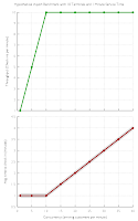 |
| Throughput and Response Time in Theory |
Going back to the first graph from the web app we see that the saturation limit is only achieved once (at 4 active connections). All consecutive results are below that. The reason for that is simple. Reaching the saturation limit of a web application means that at least one element in your architecture (e.g. the CPU of the web server or the disks of the database) have reached their saturation limit. As more and more tasks/processes/threads are competing over the limited resources the operating system is usually trying to give each of them a
fair share which in turn requires more and more
context switches. Generally the inefficiency incurred due to time spent doing context switches instead of actual work increases with the load of the system. Therefore you want to make sure that your application is running under the saturation point (i.e. at maximum efficiency and throughput). Unfortunately, on the other hand, you cannot always predict the actual traffic which is why you want to know how your application behaves beyond the saturation limit. In practice you need to know at which point an intolerable response time is reached and, even as important, at which point you application stops working at all (e.g. crash due to the lack of memory).
From Theory to Practice
I prepared a small example which shows how a performance test reflecting the former theory could be conducted. A "Hello World"
PHP application was deployed to Amazon's
PaaS service
Elastic Beanstalk using a single micro instance (no
auto scaling). In addition I used Apache's
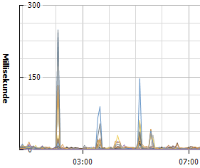
JMeter for the test. The test plan fetches the single URL for 30 seconds and records the results. The test was repeated with increased concurrency levels beyond the saturation limit until the application stopped working altogether or reached a maximum response time of 10 seconds. In order to simulate a new release deployment I ran an additional test replacing the Hello World one liner with a
small app that prints out one of the first 10
Fibonacci numbers randomly (recursive implementation). As you can see in the results the simple change has quite an impact on throughput and response time with increasing concurrency. With such results you have the chance to either optimize the application or increase the capacity
before deployment. Moreover the throughput graph is color coded by error rate. With the shown results you should not run this demo application with more than 128 active connections. If have an
application delivery controller (ADC) that is capable of multiplexing backend connections (
ELB is not) you should make sure that the configured maximum of backend connection lies beneath 128 and as close as possible to the saturation limit. This way the ADC will handle the queueing and the backend can continue to operate close to the measured peak throughput**.
 |
Occasionally Freezing Micro
Instance during Load Test |
If you try to reproduce this example you will notice that you will get different results on repeated tests. The reason for that is the use of
micro instances. The point at which the CPU is throttled varies quite a bit and therefore the results are changing. During the 30 second test there are periods where the instance seems to freeze for a few seconds. More details about this behavior can be found
here. Moreover, with higher concurrency the likeness of failed health checks form the ELB increases. I had two tests were the ELB marked the instance as unhealthy and delivered
503 error pages with no instance left. These error pages were delivered faster than the actual "Hello World" example. This is why you shouldn't trust results with errors and why those errors are color coded in the result graph.
Actual Practice
 |
| JMeter Summary Report |
The graphs shown in this blog post were created with
gnuplot using
this script. It expects CSV-files generated from the JMeter
summary report as input. Those can be provided via command line by using
gnuplot -e "datafile = 'summary.csv';" or
gnuplot -e "datafile = 'summary1.csv'; datafile_cmp = 'summary_old.csv';" for a graph comparing two results. Additionally the labels are defaulting to the provided file names. Those can be customized by setting the
datafile_title and
datafile_cmp_title variables.
The corresponding JMeter
test file is using a single thread group for each concurrency step. I decided to use powers of two for this, but you might want to add intermediate steps on higher concurrencies. Note that this test only requests a single resource (the home page). An actual application will probably consist of more URLs requiring modifications to this test plan. My preferred setup is to use the
CSV data set config element to provide a representative set of resources to test. If you run a test using this example make sure to adjust the variables from the test plan (especially the target of the performance test). After the test is done save the result using the "Save Table Data" button from the summary report. Expect that this test will render your web application unresponsive. So do not run it against a production environment.
/jr
* Due to the nature of the test we can safely assume flow balance which means that the responses per seconds are equal to the request per seconds
** This requires similar response times across all resources. A few long running scripts could block the back end connections